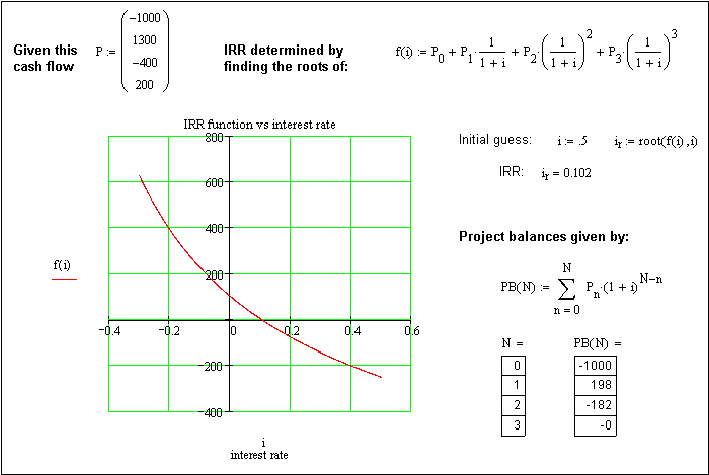
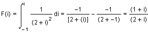
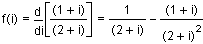
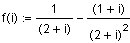
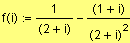
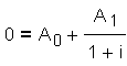
This analysis investigates the stochastic IRR problem (shown to the right) where A₀, A₁,..., A_n are cash flows (random variables) derived in this analysis from known exponential distributions. The goal is to develop the probability density function (pdf) and cummulative distribution function (cdf) for the internal rate of return (interest, i) for this investment. A deterministic example of IRR is shown below.

Only the simplest form of this problem will be considered where:

(where i is the interest rate)

The PDF, CDF and mean for two cases of this basic problem are determined.

Example

Page 3

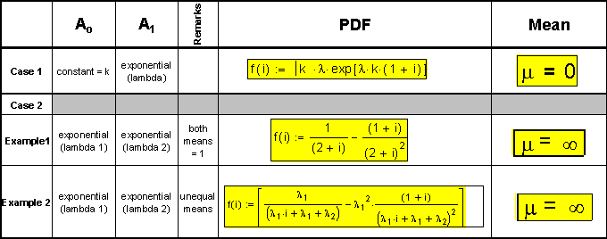
Case 1 - A₀ is a constant (fixed initial investment) and A₁ is a random variable derived from an exponential distribution with a know mean.

Page 9

Case 2 - A₀ and A₁ are both random variables.
Two examples are considered:

Page 14

Example 1 - both random variables distributions are derived from exponential distributions having the same means.

Example 2 - random variables are derived from exponential distributions with differing means.

Page 21

See the page 27 for a summary of the equations for resulting distribution PDFs, CDFs, and means
as a function of the interest rate (i).

Case 1 - A₀ is a constant

For the problem:

Can y = 1 + i ?
Yes if the relationship is multiplied by or is added to by a constant... See Shooman's text, page 394, # 1 and # 2. To get f(i), see transformations at end of this Case 1 analysis.

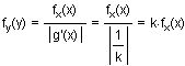
Letting y = 1 + i, A₀ = k, A₁ = x, where k is a constant, x and y are RVs, the problem becomes:

or

Determine the probability density function (PDF) for the random variable y given that x is derived from an exponential distribution.

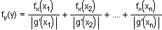
Using the fundamental theorem (From A. Papoulis text, page 95, Probability, Random Variables, and Stochastic Processes, 1984, ISBN 0-07-048468-6):

Given a probability density function f_x(x), to find f_y(y) for a specific y, we solve the equation y = g(x), where g(x) denotes the relationship between the random variables. Denoting it's real roots by x_n

Letting

Determine y, given x and y are related random variables (with x derived from some distribution and k is a constant).

For Case 1

( remembering for our IRR problem y = 1 + i )

thus

or

or

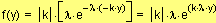
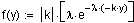
The equation y = - x / k has a single solution at x = - k * y. Applying the fundamental theorem:

For the exponential distribution:

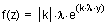
The PDF for y becomes:

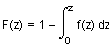
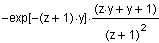
Checking to seem if f(y) is a valid PDF for 0 < y < ¥ where k is some negative constant (since for our IRR Problem, k represents A_o or some initial investment (negative) at the first period 0):

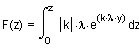
Integrating the PDF numerically and checking the result using a large y.

Computing the mean for this specific problem (remembering l = 1 and k = -1):

(when y = 1 + i)

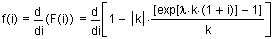
Changing the distribution from f(y) to f(i) where y = 1 + i where i is the interest rate (per the discussion 3/25/02).

Case 1 - A_o is a constant and A₁ is exponentially distributed.

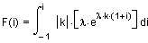
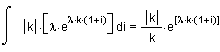
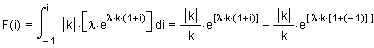
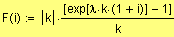
original limits of integration

substitution since z =1 + i

new limits for i

remembering

making a change in variables:

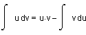
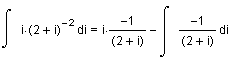
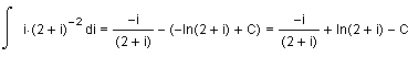
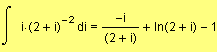
where the indefinite integral is:

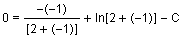
calculating the CDF for i using the new limits

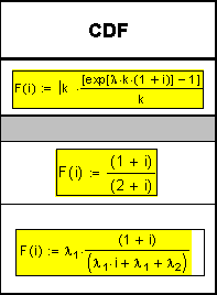
the CDF simplifies to:

(CDF)

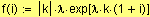
calculating the PDF for i

or

(PDF)

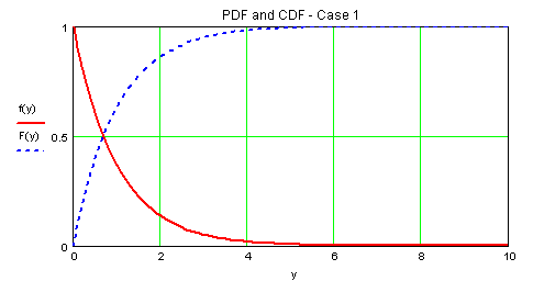
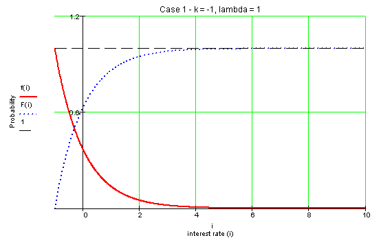
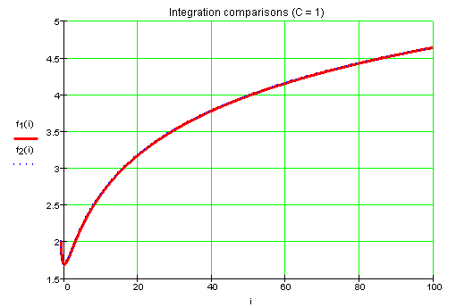
remembering l = 1 and k = -1 and graphing the PDF and CDF over the domain:

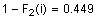
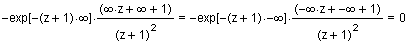
Confirming the CDF = 1:

(m = 0 since k = -1 and l = 1)

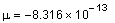
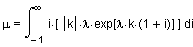
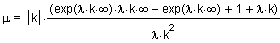
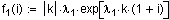
Calculating the mean for Case 1.

Using the pdf developed on the previous page:

The mean is defined as:

Integrating yields:

or

Case 1 - What does this all mean? Remembering Case 1 is the problem to the right where A_o is a constant (a known investment) and A₁ is a single payment ( to repay the investment) derived from an exponential distribution with a known mean. Consider the following example:

Suppose two companies desire a $10,000 investment, each with different mean for a single payment derived from exponential distribution:

Money invested

Company A

Company B

Assume you wish to have an IRR of exactly 20%.

Probability

Company A

Company B

Assume the IRR must be greater than 20%.

Probability

Company A

Company B

Company B appears to be the better choice to invest in! Of course, we knew that since it had a greater mean.

Case 2 - A₀ and A1 are both random variables drawn from different exponential distributions.

For the problem:

Letting x = (1+i), where A₀ and A₁ are RVs, the problem becomes:

Determine the probability density function (PDF) for the random variable x given that A₀ and A₁ are derived from exponential distributions.

Since this problem requires the development of a PDF that is the quotient of two random variables, a discussion of the theory is begins on the next page.

This theory is extrapolated from:

B. V. Gnedenko, The Theory of Probability; Chelsea Publishing Company, 1962, pages 185-186

A. Papoulis, Probability, Random Variables, and Stochastic Processes; McGraw-Hill Book Company, 1965

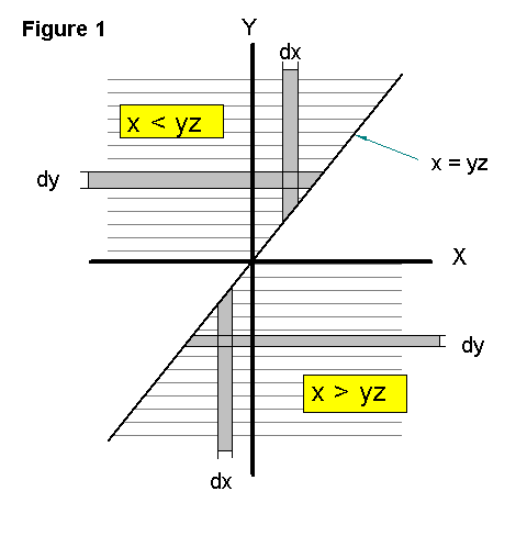
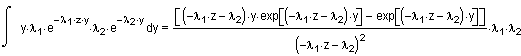
Analysis of the quotient of two random variables

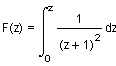
Determine the density function f(z) representing the quotient of the two independent random variables x and y derived from continuous density functions f₁(x) and f₂(y).

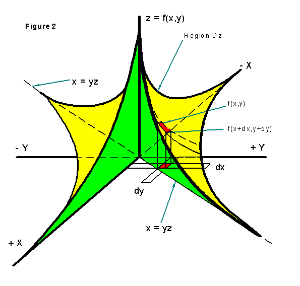
The region D_z, of the xy plane such that:

is the lined area of Figure 1 shown to the right because:

If

then

If

then

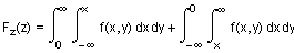
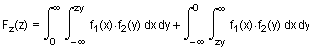
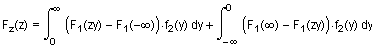
For the two random variables x and y, the masses in D_z are just the just volumes under f(z) as seen in Figure 2. The volumes under f(z) are just the CDF - cumulative distribution function F(z).

[1]

from Figures 1 and 2

[2]

since

since f₁(x) and f₂(y) are independent

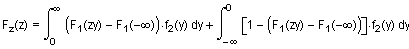
[3]

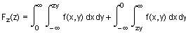
integrating the inner most terms with respect to x

[4]

but since the probabilities must sum to 1

[5]

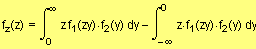
differentiating with respect to z to get the PDF probability density function f(z):

[6]

Equation [6] provides the PDF (probability density function) for the quotient of 2 random variables x and y derived from continuous, independent density functions f₁(x) and f₂(y).

Determine the probability density function f_z(z) representing the quotient of two random variables e and h derived respectively from independent exponential density functions.

Remembering, for the IRR problem: z = 1 + i (where i is the interest rate).

Equation [6] derived the general density function for the quotient of two random variables:

substitution yields:

[7]

the indefinite integral of

is

[7a]

Example 1: Letting l₁ = l₂ = 1 the indefinite integral of equation [ 7a ] becomes:

the definite integral for f_z(z) is:

since

Note: In equation [7], the left integral supports 0 < z < ¥ while the right integral supports -¥ < z < 0 .

the definite integral becomes

( for -¥ < z < ¥ )

( for 0 < z < ¥ )

[8]

(which is what is given by equation 25 on page 397 of Shooman's book)

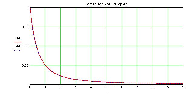
A confirmation of the analytical solution is performed below by comparing it to a numerical integration of equation [7] from 0 < z < 10 .

numerical function

analytical function

Case 1 conclusion:

for 0 < z < ¥ and l₁ = l₂ = 1,
both curves overlay indicating equation [7] is equivalent to equation [8].

Changing the distribution from f(z) to f(i) where z = 1 + i where i is the interest rate.

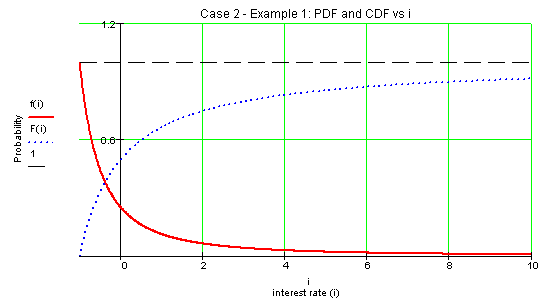
Case 2, Example 1 (exponential distributions with equal means) as derived on page 13:

( for 0 < z < ¥ )

(which is what is given by equation 25 on page 397 of Shooman's book)

Changing the independent variable to i (interest rate) since z = 1 + i

original limits of z

substitution since z =1 + i

new limits for i

remembering

making a change in variables and limits:

where the indefinite integral is:

calculating the CDF for i using the new limits

calculating the PDF for i

or

graphing the PDF and CDF

and

over the domain:

Confirming the CDF = 1:

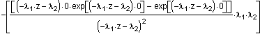
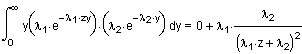
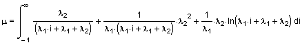
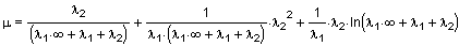
Calculating the mean of the quotient of 2 exponential distributions having equal means (1/l₁ = 1/l₂ = 1).

definition of the mean (for our PDF):

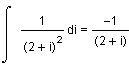
computing the indefinite integral (using Mathcad to avoid the tedious integration by parts):

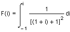
computing the definite integral using the limits: -1 to ¥ :

m = ¥

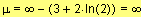
Just for kicks, let's do a hand solution and integrate:

first simplify the integrand:

thus

integrating by parts:

letting

substitution

thus

Solving for C since we know
f(-1) = 0
[the mean is zero when i = -1]:

thus

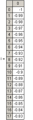
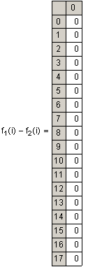
For confirmation, let's graph both the Mathcad and hand solutions to see if they're equal when:

Mathcad solution

hand solution

Difference Table for the First 17 Values

over the domain

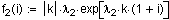
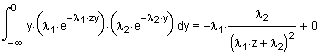
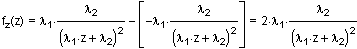
Example 2: Letting

and remembering from equation [ 7a ]:

Applying the limits of integration to the first integral in f_z(z)

since:

so...

Applying the limits of integration to the second integral in f_z(z)

since:

so...

The PDF of the quotient of two random variables derived from different exponential functions from -¥ < z < ¥ is:

( -¥ < z < ¥ )

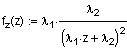
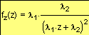
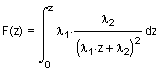
The PDF of the quotient of two random variables derived from exponential functions having different means (from 0 < z < ¥) is:

( 0 < z < ¥ )

Checking the PDF and CDF for example 2:

Checking the CDF numerically with a large number to ensure it equals 1.

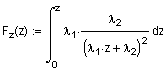
Changing the distribution from f(z) to f(i) where z = 1 + i where i is the interest rate.

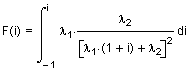
Case 2, Example 2 (exponential distributions with unequal means) was derived on pages 20 - 21:

( for 0 < z < ¥ )

Letting (for example):

Changing the independent variable to i (interest rate) since z = 1 + i

original limits of z

substitution since z =1 + i

new limits for i

remembering

making a change in variables and limits:

where the indefinite integral is:

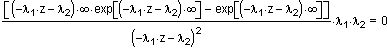
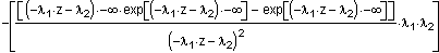
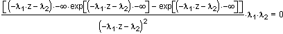
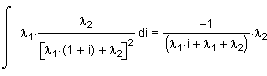
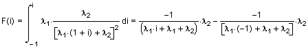
calculating the CDF for i using the new limits

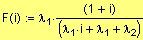
which simplifies to:

(CDF)

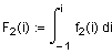
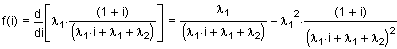
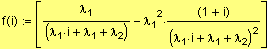
calculating the PDF for i

so

(PDF)

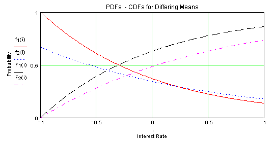
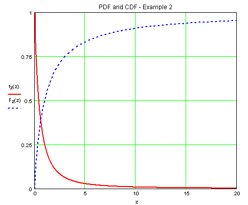
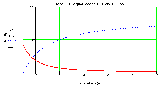
graphing the PDF and CDF (remembering l₁ = 1 and l₂ = 2) over the domain:

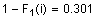
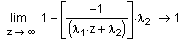
Confirming the CDF = 1:

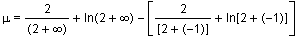
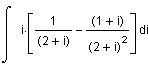
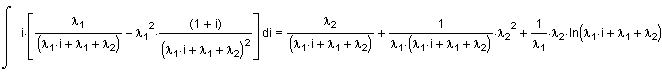
Calculating the mean of the quotient of 2 exponential distributions having unequal means.

definition of the mean (for our PDF):

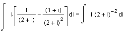
Next, computing the indefinite integral

computing the definite integral using the limits: -1 to ¥ :

or

thus

Taking the limits of both parts of the definite integral just to be sure:

Summary Page

The Investment Problem: